I wrote this essay as part of an undergraduate research project I did in 2012. Some readers might find the mathematics in some parts a little bit prickly, so I’ve marked them with an asterisk. Everything else is aimed at a general audience. I’ve also made a pretty cool hands-on workshop on fractal geometry for middle-schoolers. Get in touch if you want to chat about it.
What is a fractal?
A fractal is a geometric object (i.e. a curve or a shape) that possesses certain properties: self-similarity, infinite complexity and non-differentiability. These properties not only make the image beautiful and interesting to look at, but result in it containing some powerful mathematics which can be used in a variety of real world applications.
Self-similarity
An image is self-similar if the whole or a part of the image is repeated within itself continually at smaller scales. Take the Koch snowflake as an example.
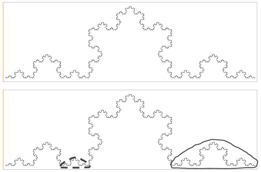
You can see that if it were iterated to infinity, the smaller sub-sections would be identical to the whole image, except scaled down. For example, the section of the curve contained within the solid line above shows a curve identical to the whole Koch curve, except scaled down to 1/3 of the original size. Similarly, the section within the dashed line shows the same whole curve again, except this time scaled down to 1/9 of the size.
Another example of this exact self-similarity is the mathematically generated fern.
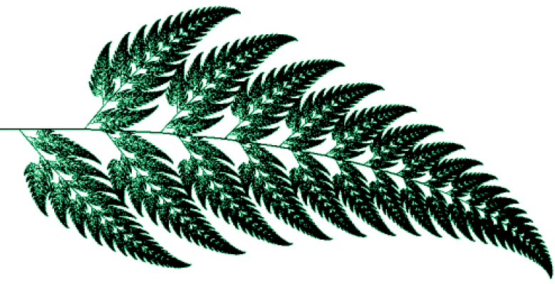
Each branch from the main trunk is a replica of the whole fern. Off the trunks of these smaller ferns stem even smaller ferns, and from these stem ever smaller ones, etc.
Self-similarity can be observed in natural systems as well, such as broccoli. If you start with a whole broccoli, and remove a branch from it, the branch will look similar to the whole broccoli. From this branch, you can remove an even smaller branch which again looks just like the whole broccoli. It’s broccolis all the way down. Of course, the smaller broccoli branches aren’t identical to the whole broccoli, but are still quite similar. This imperfect self-similarity is known as quasi self-similarity, an alternative to the exact self-similarity that was demonstrated through the Koch Curve. Quasi self-similarity occurs when the scaled down image is roughly similar to the main image, but not perfectly the same (Oldershaw 2002).
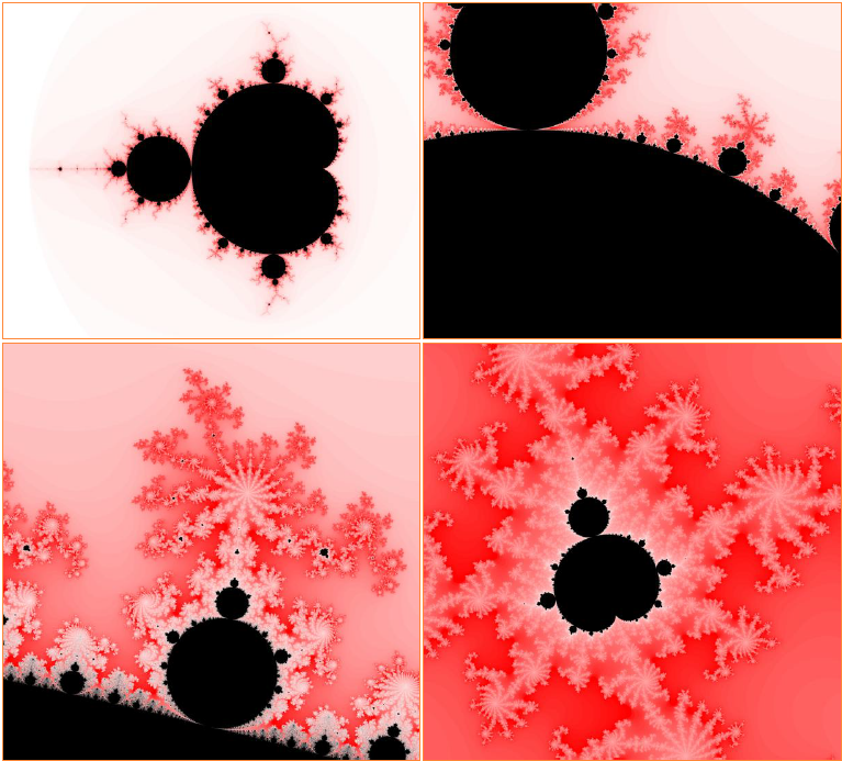
Quasi self-similarity is present in the Mandelbrot Set, shown below, but we’ll talk about him a bit more later on. The top-left image shows the entire Mandelbrot Set, and each proceeding image (top left to bottom right) zooms into a particular point in the previous image. At each zoom level, a very similar but scaled down image of the set appears within the set.
Infinite Complexity
True fractals possess infinite complexity. This means that as you zoom into the fractal there will always be more to see. It is analogous to a photo with infinite resolution. This is easy to imagine when considering a fractal like the Koch Curve. The algorithm that is used to create the image is repeated an infinite amount of times, which means that you could spend a lifetime zooming into the image and you’ll never reach the end of it (like in Blade Runner).
This idea isn’t immediately obvious with images like the Mandelbrot Set. The construction of these types of fractals will be discussed later (in Escape-Time Fractals). To explain briefly: the Mandelbrot Set is a set of points on a complex number plane (a plane with real number and imaginary number axes), where the colour of each point is determined using an algorithm (a set of mathematical rules). Because there is an uncountable infinity of points on the grid, there will always be somewhere to zoom into and find more of the fractal pattern.
Non-Differentiable*
The third property that a fractal must possess is that of non-differentiability, meaning that differential calculus cannot be applied to it. Applying differential calculus essentially means finding the gradient (or slope) at any given point of the curve. The nature of fractals, with their infinite complexity and fairly unpredictable nature, means that there is no point on the fractal where an appropriate tangent can be drawn to calculate a gradient.
The discovery of the Weierstrass function by Karl Weierstrass in 1872 marked a big change to the notion of non-differentiability (Lesmoir-Gordon, Rood & Edney 2000). Here’s an example of a Weierstrass function:
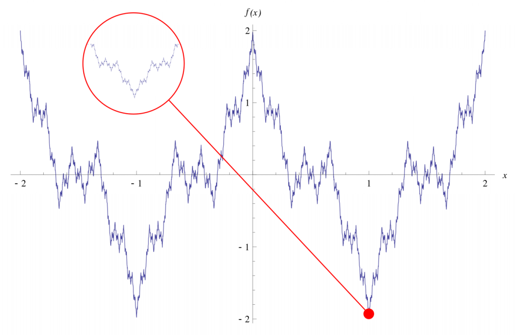
The discovery of this function was a turning point in mathematics (pun) as it was the first function to be created that was continuous but not differentiable. The Weierstrass function actually has many variations, all non-differentiable. Every point on the function will be next to two points that are either both below it or both above it: this means that it is entirely made of turning points (Conroy 2012). The further you zoom in, the more this pattern appears. This creates one very hectic zigzag described by this equation:
Every point on the Weierstrass function is a result of an infinite sum of functions (involving an exponential and cosine function). The general form of a cosine function can be seen in the zoomed out curve, albeit very spiky. This cosine function is embedded in the self-similarity of the curve at all scales. Every y-value shown in Weierstrass function above would indicate where the infinite sum converges for that value of x. Perhaps it is the combination of the exponential and cosine function that cause this function to be so infinitely sensitive. Regardless, this function is categorized as a pathological function, which, in mathematics, means that it is counter-intuitive and difficult to work with. The opposite of a pathological function is a ‘well behaved function’ (makes sense). During the founding years of fractal geometry, fractals were referred to as ‘monsters’ which seems to appropriately reflect the frustrations that mathematicians were experiencing when dealing with such infinite, complicated systems.
Making fractals
If you’re reading this article, you’ve probably spent many nights Googling ‘fractals’ and scrolling through the endless types the internet has to show you. Here, the two main types of fractal generation will be discussed; iterated function systems and escape-time fractals.
Iterated Function Systems
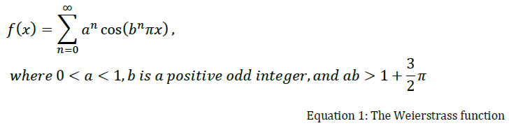
Iterated function systems (IFSs) use recursive relations to repeatedly perform an algorithm on a shape or pattern to create a fractal. For the purposes of understanding this term, the word ‘function’ is better replaced with ‘algorithm’ as that more appropriately reflects the use of IFSs in fractal geometry. For the result to be a true fractal, the algorithm must be iterated an infinite number of times. A basic IFS is demonstrated below, in the geometric construction of a simple fractal called the Sierpiński Triangle.
In this system, the initial shape is a solid equilateral triangle. The algorithm that is being performed on the shape splits the solid triangle into four smaller triangles and removes the middle triangle. This process is then repeated on all the remaining triangles infinitely.
The Sierpiński Triangle was first published by Wacław Sierpiński in 1915; however the simple design has been used in architecture from as early as 1104 AD. The triangle also has powerful links to other areas of mathematics, such as Pascal’s Triangle and Chaos Theory (Sala 2000, Weisstein 2012a).
Here are some more examples of simple IFSs, as well as the Koch Snowflake and fern from earlier.
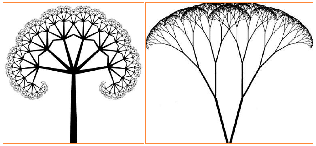
Fractal Trees
A fractal tree is one of the easiest types of IFS to understand. A standard fractal tree begins with a trunk, of length r (where 0 ≤ r ≤ 1), as the base. The end of this trunk is then split into a number of branches of length r2. These branches then spilt into the same number of branches scaled down by r again, and this process is continued to infinity.
Variations can be made to this simple system by altering:
○ the number of branches sprouting from the end of a section,
○ the value of r
○ the ratio of how much the length changes at each step
○ the angle of the splitting of branches (different branches can even branch off from the trunk at different angles)
○ incorporating a random element into the algorithm
Computer programmers can easily program a fractal tree in three dimensions (as you will read later, the fractal may have a non-integer dimension, but would be mapped on a three-dimensional plane). Leaves can also be added to these images to give the appearance of real trees: these can be used in video games and movies.
A binary tree is the most commonly used type of fractal tree. In a binary tree, every iteration produces two sub-branches per branch. Many natural systems are binary trees taken to a finite amount of iterations. Such systems include lungs, retinas, lightning and trees (Taylor 2006). Binary trees are used extensively in graph theory and computer programming to plot information or probabilities. They also form the structure of computer hardware.
Binary trees can be defined as either self-avoiding (no branches intersect with each other) or self-contacting (the branches cross) (Taylor 2006). Rules can be created to determine what happens in the construction of a binary tree if an intersection is made. For example, starting with a standard binary tree with a branching angle of 60 degrees, a rule can be set that if two branches intersect, the branches cease at that point and the closed-in shape formed by the intersection gets coloured in. This system, such a simple set of rules, taken to an infinite number of iterations, creates the Sierpiński Triangle (Hart 2012).
Escape-Time Fractals
Escape-time fractals could also be considered iterated function systems, as they rely on recursive relations to determine their shape. The difference here however, is that the recursive relation is performed on every point of a space (commonly the complex number plane) to determine whether or not that point is in a set. A point is in the set if it conforms to certain mathematical boundaries. Two of the most popular examples, the Mandelbrot Set and the Julia Set.
Mandelbrot Set*
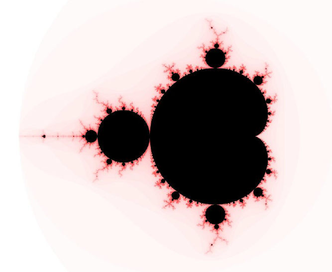
The Mandelbrot Set was named after Benoît B. Mandelbrot, who is widely regarded as the father of modern fractal geometry. The Mandelbrot Set is a set of complex numbers that abide by a certain mathematical rule. This rule is as follows:
Let c be the complex number in question. If this number is substituted into the recursive relation, zn+1 = zn2+c , where z0 = 0+0i, a new value for zn+1 will be produced with every iteration. For some values of c, the values for will sky rocket off to infinity (said to ‘escape’). For some values of c, however, the values will settle to within a small range, or sometimes a single number. These values are said to ‘converge’, and are what make up the Mandelbrot Set. Generally, if the value of ever exceeds two, it is said to escape the set (there is some strong mathematics behind the choosing of this number but is not relevant here).
When generating an image of the Mandelbrot Set, the colours or shading of the image are produced by applying a gradient that corresponds to how many iterations are required to be performed before each number escapes or converges. In Figure 8, below, the black points represent numbers that are in the Mandelbrot Set, and the white points around the edges indicate that the number escapes very fast. As you approach the border of the Mandelbrot Set, the colour of the points become red and get progressively darker, indicating that a lot more iterations are required for the number to escape.
Little known fact about Benoit B. Mandelbrot: the “B” stands for Benoit B. Mandelbrot…
Julia Set*
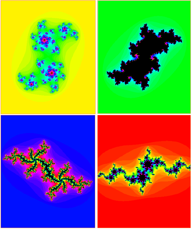
The Julia Set uses a recursive relation very similar to the one used for the Mandelbrot Set. However, the Julia Set is actually a set of infinite sets.
To generate a single Julia Set, use the equation zn+1=zn2+c and select a value for c. This value is known as the ‘seed’ and is the number associated with the set that will be generated. From there, every number on the complex plane is used individually as a starting value for and the recursive relation is performed (using the seed value for c) to again determine whether or not the number escapes or diverges (Bourke 2001). An image is normally produced, using a similar colouring method to the Mandelbrot Set.
As mentioned previously, there are an infinite number of subsets within the whole Julia Set, each associated with a different value for c. Since there are two imaginary numbers involved (zn+1 and zn), each with two components (real and imaginary), by altering the combination of the components used as the seed, even more subsets can be created (Bourke 2001). This, however, is far beyond the scope of this essay; as it enters the fourth dimension, and that requires a great deal of wibbly-wobbly timey-wimey stuff. So let’s move on.
Below are some images of various Julia Sets, and their associated starting values of c.
Characteristics of a fractal
The nature of fractals lead to them having a certain ‘roughness’ about them. This roughness is what was lacking from traditional Euclidean geometry when it was used to describe objects and systems in nature. For example, as Mandelbrot (1982) stated, “clouds are not spheres, mountains are not cones”. These natural objects have a fractal-like nature about them, and mathematicians have developed ways to characterise them, using quantitative methods. This can be used to assess the general nature of a fractal, as well as compare it to another fractal. The two main characteristics of a fractal are its fractal dimension and its lacunarity.
Fractal dimension
The concepts of regular geometric dimension are familiar to most people. A cube is three-dimensional, a square is two-dimensional, and line is one-dimensional, and a point has no dimension. Because there is a certain roughness associated with most fractals, their dimensions are often calculated to be non-integer (i.e. not a whole number). Let’s explore that.
Before any iterations are made, the Koch Snowflake is a line. As it is constructed (remove the middle third of the line, replace this with two lines of the same length to make a triangle, repeat on all lines), it covers more area. The Koch Curve has a fractal dimension of approximately 1.26, which you can sort of rationalise because it starts as a one-dimensional line and moves into a two-dimensional area (Weisstein 2012b). Because 1.26 is closer to 1 than 2, it can be said that the curve is closer to being a line than an area.
If the curve was rougher, causing it to cover more area, the fractal dimension would be closer to two. In fact, there is a class of fractals called “space filling curves” (Gross 2007). The first of its kind, the Peano Curve, is shown in stages below.
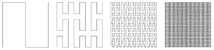
The curve starts as a line (one-dimension), but the nature of its algorithm causes it to fill more space with every iteration. When this iteration is taken to infinity, it fills up an entire square (two-dimensions). It’s like a mathematical crayon! For this reason, the curve is said to have a fractal dimension of two (Gross 2007).
While the Koch Curve and Peano Curve both start as lines and build up into a higher dimension, some fractals start at a higher dimension and break down into a lower one. For example, the Sierpiński Triangle (Figure 5) starts as a solid two-dimensional shape and as parts are removed, with every iteration, it begins to resemble a collection of lines. The Sierpiński Triangle has a fractal dimension of 1.59 (Weisstein 2012a).
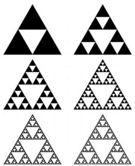
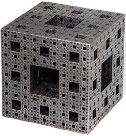
Of course, fractal dimension isn’t restricted to fractals between one and two dimensions. The Cantor Set (Figure 6) starts as a line and breaks down, meaning it has a fractal dimension between zero and one. The fractal dimension of the Cantor Set is 0.63 (Weisstein 2012c). The Menger Sponge (Figure 11, below) starts as a cube and has sections removed, resulting in a fractal dimension of between two and three (Weisstein 2012d).
You can learn how to calculate the dimension of a fractal here.
Lacunarity
Lacunarity is a measure of the distribution of the fractal, depending on where there are gaps in the shape. More formally, lacunarity is a measure of the translational and rotational variance (Sengupta & Vinoy 2006). This means it is a measure of how much an image changes when you rotate or slide it. Lacunarity measures (at a given scale) how similar different parts of a shape are to each other (Sengupta & Vinoy 2006).
Lacunarity is highly dependent on the scale it is measured on. Typically, a ‘sliding box method’ is used. In this method, boxes of different sizes are used, and the amount of space this box is filled by the fractal at various locations is recorded. The larger the box, the more of the shape’s gaps would be missed. Typically, to compare the lacunarity of two fractals, a plot of their lacunarity for various box sizes would be made, and then the parameters of the produced curve would be calculated and used to compare different fractals (Sengupta & Vinoy 2006).
Similarly to fractal dimension, there is no ‘golden method’ for calculating lacunarity that can be applied in all cases, as all fractals have different properties and patterns.
Fractal dimension vs. lacunarity
Fractal dimension and lacunarity are not necessarily correlated. While they are commonly associated with one another, they measure two different properties of fractals: the roughness, and the distribution of a fractal. Two fractals with the same fractal dimension could look completely different because they have a different lacunarity, and vice versa. Fractal dimension and lacunarity can be used to categorise and characterise a fractal.
Chaos theory
Chaos theory is a field of mathematics that is commonly associated with fractal geometry, mostly due to its presence in popular culture. Chaos theory is the study of systems that change over time which are highly sensitive to minuscule changes in their starting positions (Weisstein 2012e). This effect is commonly known as the ‘Butterfly Effect’, named after the analogy of a butterfly flapping its wings which starts a train of events eventually resulting in a hurricane on the other side of the world. Of course, this analogy isn’t accurate, as fierce weather systems are not dependent on tiny insects, however it is used to demonstrate the effect of such a small disturbance to starting conditions initiating a string of events that eventually get wildly out of control and produce an unpredictable result.
Even if a system is entirely deterministic (i.e. every action or iteration is completely dependent on the previous conditions and no random elements are involved) a system can still get wildly out of control (University of Arizona 2003). For example, a swinging double pendulum system is deterministic as every movement is based on momentum, acceleration, gravity and other factors. However in motion (like this video) the actions of the double pendulum become quite unpredictable. A small change to the initial starting position of the double pendulum results in it taking an entirely different path (University of Arizona 2003). In fact, a plot of the time taken for the double pendulum to flip over, as a function of initial starting conditions, results in the graph shown below (University of Arizona 2003).
An important aspect of Chaos Theory is that even though a system might be entirely deterministic, even by being given a final product of a system and knowing all the rules associated with it, it would be impossible to back track and determine the starting conditions (Weisstein 2012e).
Cellular Automata
A cellular automaton (CA) is a discrete model used to simulate various real-world systems. Cellular automata (plural) use a grid of cells to represent an environment, and each cell exists in particular state (e.g. on/off, black/white, human/infected/zombie). A certain set of rules govern the system, and these rules are applied to every cell simultaneously over a number of iterations (Weisstein 2012f). Generally, these rules dictate the state of a cell in the next iteration based on the ‘neighbourhood’ of the cell in the previous iteration. Here, the neighbourhood consists of the cell and all cells within a specified distance from that cell (similar to the system used in the game Minesweeper) (Weisstein 2012f).
An example of a rule could be: The cell is “on” in the next generation if exactly two of the cells in the neighbourhood are “on” in the current generation; otherwise the cell is “off” in the next generation.
A famous CA is Conway’s Game of Life, created in 1970 and named after its creator John Conway (Callahan 2010). The possible states for the cells in this CA are ‘dead’ (white) or ‘alive’ (black). The rules that govern the system are as follows:
○ Any live cell with fewer than two live neighbours dies, as if caused by under-population.
○ Any live cell with two or three live neighbours lives through to the next generation.
○ Any live cell with more than three live neighbours dies, as if by over-population.
○ Any dead cell with exactly three live neighbours becomes a live cell, as if by reproduction.
(Callahan 2010)
The user of the Game of Life can adjust the starting conditions by deciding what cells are alive or dead. From there, the iterations start, and the rules are applied to the system. Have a go. A small change in the starting conditions lead to completely different outcomes which, although are entirely deterministic, means that it is impossible to work backwards through the iterations to determine the starting conditions. This sort of function is called a ‘Trapdoor Function’, which can be computed in one direction but not the other (Callahan 2010).
The simplest type of CA is a binary system (two possible states) in a one-dimensional grid (a single row of cells). This is called an elementary cellular automaton (Weisstein 2012f). Since it is one dimensional (i.e. a line), a cell can only have a neighbourhood of 3 (including original cell). Each of these cells can have one of two states, resulting in 23, or eight, different combinations for a neighbourhood (Weisstein 2012f). Since a rule defines the state of the cell based on its previous neighbourhood, of which there are eight different combinations,, and there are two options for its new state, the number of rules possible in this situation is 28, or 256, rules (Weisstein 2012f).
Stephen Wolfram (i.e. the guy who made Wolfram Alpha, a mathematically-thinking search engine) developed a system for identifying the effects of each of these rules. They are referred to by their Wolfram Code, a number between 1 and 256. Each Wolfram Code has a map associated with it, starting with a row with a single “on” (black) cell, and each successive row underneath it depicts the next iteration. Various Wolfram Codes have been selected as codes of interest, for example Rule 30 (below) has been flagged for its almost random behaviour which has strong applications in cryptology (Weisstein 2012f).

Each rule creates a different image, of all shapes and forms. Many of these rules create fractal systems, such as Rule 90 which creates the Sierpiński Triangle.

It should be noted that while CA are discrete systems, if they are iterated an infinite number of times and displayed like the previous two images, they can possess infinite complexity and therefore be fractals.
A key idea behind cellular automata is that such a simple premise can create something so complex and seemingly unpredictable. Wolfram applied this idea to nature, suggesting that the complexity of the natural world could be described by a few simple rules and initial conditions (Wolfram 2002).
‘Digital physics’ describes the theory that everything in the physical world can be described using information and is therefore computable (Wolfram 2002). Essentially, our entire universe could potentially be a huge amount of information governed by a few physical rules (although in such a system, there would be more complexity than just ‘on’ and ‘off’ states).
After reading and absorbing this summary of fractal geometry, I hope you go outside and feel overwhelmed by the abundance of fractal systems that are all around you. You will stare at a tree and see the binary tree system of its branches. In that tree will be a bird, which contains fractals in the structure of its lungs and vein systems. Nearby a butterfly will flap its wings, perhaps starting a chaotic chain of events (but hopefully it won’t start a hurricane). The world is not perfectly smooth, nor is it predictable. Fractal geometry strives to define real world systems, and recreate order in the chaos of the universe.
References
Author Unknown 2003, What is Chaos?, lecture one, University of Arizona, USA, viewed 1st April 2012, http://math.arizona.edu/~shankar/efa/efa1
Bourke, P 2001, Julia Set Fractal (2D), viewed 6th May 2012, http://local.wasp.uwa.edu.au/~pbourke/fractals/juliaset/
Lesmoir-Gordon, N, Rood, W & Callahan, P 2010, What is the Game of Life?, viewed 23rd March 2012, http://www.math.com/students/wonders/life/life.html
Conroy, M 2012, Weierstrass functions, University of Washington, USA, viewed 9th June 2012, http://www.math.washington.edu/~conroy/general/weierstrass/weier.htm
Edney, R 2000, Introducing Fractal Geometry, Icon Books Ltd., Cambridge. Lowther, G, Krowne, A, matte, Sanchez, P & Woo, C 2009, nowhere differentiable, version 20, PlanetMath.org, http://planetmath.org/WeierstrassFunction.html
Gross, A 2007, Unconventional Space-filling Curves, The University of Chicago, USA, viewed 8th June 2012, http://www.math.uchicago.edu/~may/VIGRE/VIGRE2007/REUPapers/FINALAPP/Gross.pdf
Hart, V 2010, Doodling in Math Class: Binary Trees, video, viewed 7th June 2012, http://www.youtube.com/watch?v=e4MSN6IImpI
Mandelbrot, B 1982, The Fractal Geometry of Nature, Macmillian, USA.
Oldershaw, R 2002, Nature Adores Self-Similarity, Amherst College, USA, viewed 24th February 2012, http://www3.amherst.edu/~rloldershaw/nature.html
Riddle, L 2010, Classic Iterated Function Systems, viewed 11th March 2012, http://ecademy.agnesscott.edu/~lriddle/ifs/ifs.htm
Sala N 2000, Fractal Models in Architecture: A Case of Study, University of Italian Switzerland, Switzerland, viewed 1st April 2012, http://math.unipa.it/~grim/Jsalaworkshop.PDF
Sengupta, K & Vinoy, KJ 2006, ‘A new measure of lacunarity for generalized fractals and its impact in the electromagnetic behavior of Koch dipole antennas’, Fractals, World Scientific Publishing Company, http://www.its.caltech.edu/~kaushiks/KS_Fractals.pdf
Taylor, T 2006, Fractal Trees, Topology and The Golden Ratio, MS PowerPoint presentation, St. Francis Xavier University, Canada.
Weisstein, E 2012a, Sierpiński Sieve, viewed 1st April 2012, http://mathworld.wolfram.com/SierpinskiSieve.html
Weisstein, E 2012b, Koch Snowflake, viewed 1st April 2012, http://mathworld.wolfram.com/KochSnowflake.html
Weisstein, E 2012c, Cantor Set, viewed 1st April 2012, http://mathworld.wolfram.com/CantorSet.html
Weisstein, E 2012d, Menger Sponge, viewed 1st April 2012, http://mathworld.wolfram.com/MengerSponge.html
Weisstein, E 2012e, Chaos, viewed 29th March 2012, http://mathworld.wolfram.com/Chaos.html
Weisstein, E 2012f, Cellular Automaton, viewed 23rd March 2012, http://mathworld.wolfram.com/CellularAutomaton.html
Wolfram, S 2002, A New Kind of Science, Wolfram Media, USA.
Images
Zoom of the Mandelbrot Set http://upload.wikimedia.org/wikipedia/commons/f/fc/Mandel_zoom_08_satellite_antenna.jpg
Koch Curve demonstrating self-similarity. http://www.jimloy.com/fractals/koch0.gif
Mathematically generated fern. http://www.stsci.edu/~lbradley/seminar/images/fern.gif
The Mandelbrot Set depicted at different zoom levels to demonstrate quasi self-similarity. Images generated and supplied by Dr. Aaron N Wiegand, University of the Sunshine Coast.
The Weierstrass Function, the first non-differentiable function. http://upload.wikimedia.org/wikipedia/commons/thumb/6/60/WeierstrassFunction.svg/300px-WeierstrassFunction.svg.png
Construction of Sierpiński Triangle, demonstrating an iterated function system. http://acunix.wheatonma.edu/jsklensk/Art_Spring09/inclass/fractals/sierptristeps1thru6.jpg
The Cantor Set (left) and Apollonian’s Gasket (right), both illustrating iterated function systems. http://local.wasp.uwa.edu.au/~pbourke/fractals/gasket/gasket1.gif
http://en.wikipedia.org/wiki/File:Apollonian_gasket.svg
Examples of fractal trees http://i275.photobucket.com/albums/jj296/Three_Dee/FractalTreePreset1.jpg
http://www.rupert.id.au/fractals/lesson/images/fractal-tree.jpg
Various Julia Sets with different seed values: (-0.38+0.40i), (0.047+0.64i), (0.49-0.61i), and (1.04+0.26i). http://aleph0.clarku.edu/~djoyce/cgi-bin/expl.cgi
Peano’s space-filling curve http://upload.wikimedia.org/wikipedia/commons/5/58/Peano_curve.png
The Menger Sponge, and iterated function system with a fractal dimension of 2.73. http://www.daviddarling.info/images/Menger_sponge.jpg
The fractal like image produced by changing the initial starting position of a swinging double pendulum.
http://upload.wikimedia.org/wikipedia/commons/8/87/Double_pendulum_flips_graph.png
The cellular automaton created by applying Rule 30 (Wolfram Code). Each row represents the successive iterations when the rule is applied to a row with a single ‘on’ cell. http://upload.wikimedia.org/wikipedia/commons/9/9d/CA_rule30s.png
The cellular automaton created by applying Rule 90. The image is a variation of the Sierpiński Triangle. http://mathworld.wolfram.com/images/gifs/sier90.jpg